A First Screen of 31 Anti-GFP Nanobodies
31 VHH-Fc constructs against four GFP-family proteins on SPRneo: 124 interactions from one request, about 30 hours unattended. A first screen in collaboration with DPtx.
Adam Miles, Instromeda · Nikolay Dobrev, DPtx
Summary
This note shows what one common binder-design experiment looks like when the instrument does the experimental work. 31 VHH-Fc constructs were measured against four GFP-family proteins on SPRneo: 124 interactions, set up from one request and run unattended in 29 h 57 min. The machine designed the assay, ran it and analyzed the data. The only thing people did was make the samples. 87 interactions gave a usable kinetic fit, two independently prepared batches of the same target agree to a median 1.13x in KD and 1.02x in off-rate, and the specificity profile lines up with the published co-structures down to individual residues. The same experiment can be asked for by an AI agent: ten of twelve current models designed it correctly through the instrument's MCP server, in a median of two tool calls. This is the screen that opened the project; the notes on the data below cover what to keep in mind.
Why we did this
A realistic design-and-test round. Design groups can now generate thousands of binders in silico, and typically advance a few dozen to the bench. For a therapeutic program each of those has to be tested against more than one form of the target, for example human, mouse and cynomolgus. A few dozen binders against a handful of related targets is the shape of this panel: 31 nanobodies against four GFP variants.
A familiar target with something to build on. GFP is an eleven-strand beta barrel: well understood, and not an easy design target. Published binders already exist, including the LaG series from the Rout and Chait labs 1, 2, vhhGFP4 3 and the GFP Enhancer and Minimizer 4, several with co-structures. That gives the generative stages of the project a starting point to build on. We would welcome generative designs against this target from other groups, and we can make and measure them.
A division of labor. For decades the operator of an SPR instrument has had to be the expert in everything: designing the assay, running the machine and analyzing the data. We think that is the wrong place for the skill. Here the instrument owns the experiment. It designs the assay from a request, runs it deterministically, and grades its own data, and it exposes every stage through clean interfaces (REST, MCP and SiLA 2). A scientist, an informatics system or an AI agent can work with it at any of those stages. Connecting SPRneo to DPtx's own informatics platform took about an hour, with no drivers or connectors.
Why mammalian Fc fusions first. We designed this format into the matrix on purpose: it was the one most likely to work across this set of sequences, and Fc fusions from mammalian supernatant are still a common format for nanobodies. The targets are monovalent, so a bivalent ligand on the surface still binds them one to one. Production is DPtx's expertise, and the wider project compares how the same nanobodies behave across expression routes: bacterial, cell-free and mammalian, with different tags and capture formats. Too often a company takes one production method for a set of sequences and runs with it. This screen was the first look at the panel: are the reagents active, do they bind, and what are we dealing with.
The formats in the wider project are below. This screen used the mammalian Fc format.
| Format | Expression | Construct (N to C) | Tag | Purification or capture | Role in SPR |
|---|---|---|---|---|---|
| Periplasmic VHH | E. coli | pelB - VHH - linker - 3C - Twin-Strep | Twin-Strep-II | Strep-Tactin XT resin | Ligand or analyte |
| Cytosolic VHH | E. coli (SHuffle / Origami) | VHH - linker - 3C - Twin-Strep | Twin-Strep-II | Strep-Tactin XT resin | Ligand or analyte |
| Cell-free VHH | Cell-free expression | T7 - VHH - linker - 3C - Twin-Strep | Twin-Strep-II | Direct capture, no purification | Ligand |
| Mammalian Fc (this screen) | HEK / CHO | signal - VHH - 3C - hinge - IgG1 Fc | IgG1 Fc | Protein A/G | Bivalent ligand |
| Mammalian Twin-Strep | HEK / CHO | signal - VHH - linker - 3C - Twin-Strep | Twin-Strep-II | From medium, Strep-Tactin XT | Ligand or analyte |
| Target (GFP variants) | E. coli or mammalian | FP - linker - 3C - Twin-Strep | Twin-Strep-II | Strep-Tactin XT | Ligand or analyte |
Every format carries a 3C cleavage site, for assay flexibility. The Twin-Strep formats can be run in both directions, with the nanobody on the surface or in solution, to show the same kinetics from either orientation. The Fc dimers can be run as analytes, to show avidity directly. That is why assay design matters, and why the instrument should help with it. The full study was designed around five fluorescent proteins: sfGFP, eGFP, ECFP and EYFP, plus mNeonGreen as a negative-control target, which comes from a different lineage and which the panel should not bind. This screen used three of them (sfGFP, eGFP and ECFP).
Measurement standards should come from the instrument. Several groups have recently written their own rules for when a designed binder counts: Xaira on "progressable" binders 13, Boltz on separating screening hits from confirmed binders and on what a clean sensorgram looks like 14, the wet-lab notes for Anthropic's protein binder design dataset 15, and OpenBind on releasing affinity and kinetics data with per-cycle fits 16. They agree on a lot: state the valency and orientation, treat avidity-inflated affinities as apparent, confirm ambiguous binders with a flipped or orthogonal assay, and release the sensorgrams. We do not think every group should have to invent this. The instrument's job is to get the data: given good samples, it should deliver clean kinetics, or tell the user exactly what to change to get them. An instrument that does not understand the data it generates cannot reliably give its users high-quality results. We think the only way to autonomous labs is the hard, unglamorous work of encoding those details in the instrument, and making them discoverable and legible to the people and agents who use it. We take discoverability and legibility very seriously. SPRneo grades every interaction against a fixed set of checks and keeps the verdict with the number. It reports off-rates below its floor as limits, using the same 5% dissociation rule Boltz proposes, and flags multiphasic curves rather than fitting through them. Binding data in a release is often labeled representative, with the final measurements still to come. We want to go straight to the final data: the numbers in this note come from all 124 interactions as measured and graded, including the ones that did not work.
DPtx produced all of the reagents. The method, the run and the analysis were done on SPRneo.
Materials
| What | Amount | |
|---|---|---|
| Ligands | 31 VHH-Fc constructs (human IgG1 Fc), mammalian expression (HEK/CHO), used directly as supernatant diluted 10-20x: 25 LaG clones, vhhGFP4, GFP Enhancer, GFP Minimizer, a LaG-16-LaG-2 tandem, and two negative controls (Fc only, an anti-HSA VHH-Fc) | 295 µL supernatant per construct; expression not quantified |
| Analytes | sfGFP 6, eGFP, and ECFP 7 from two independent preparations | 3-fold series, 12.3 nM to 1 µM; about 43 µg of each protein prepared |
| Surface | Protein A/G sensor chip (Xantec) | |
| Regeneration | 10 mM glycine-HCl, pH 2.0; pH 1.5 for conditioning |
We did not measure expression levels for the supernatants, and they varied a lot. The capture step tells you how much each one delivered: capture levels ranged from 28 RU to 1,582 RU, about 57-fold.
Methods
The request
The experiment is a single request: the objective (binding kinetics), the ligands and how they attach (Fc capture on a Protein A/G chip), the analytes and their concentration range. Everything else, from the method and plate layout to the dilutions, conditioning, controls and evaluations, is generated by the platform.
This run was built in the web builder. The same experiment can be asked for as a plain request, as one MCP tool call, or as one REST call. All three are below. The plain request is exactly what the models in the agent benchmark further down received; the MCP and REST calls were each checked with a preview call that saves nothing.
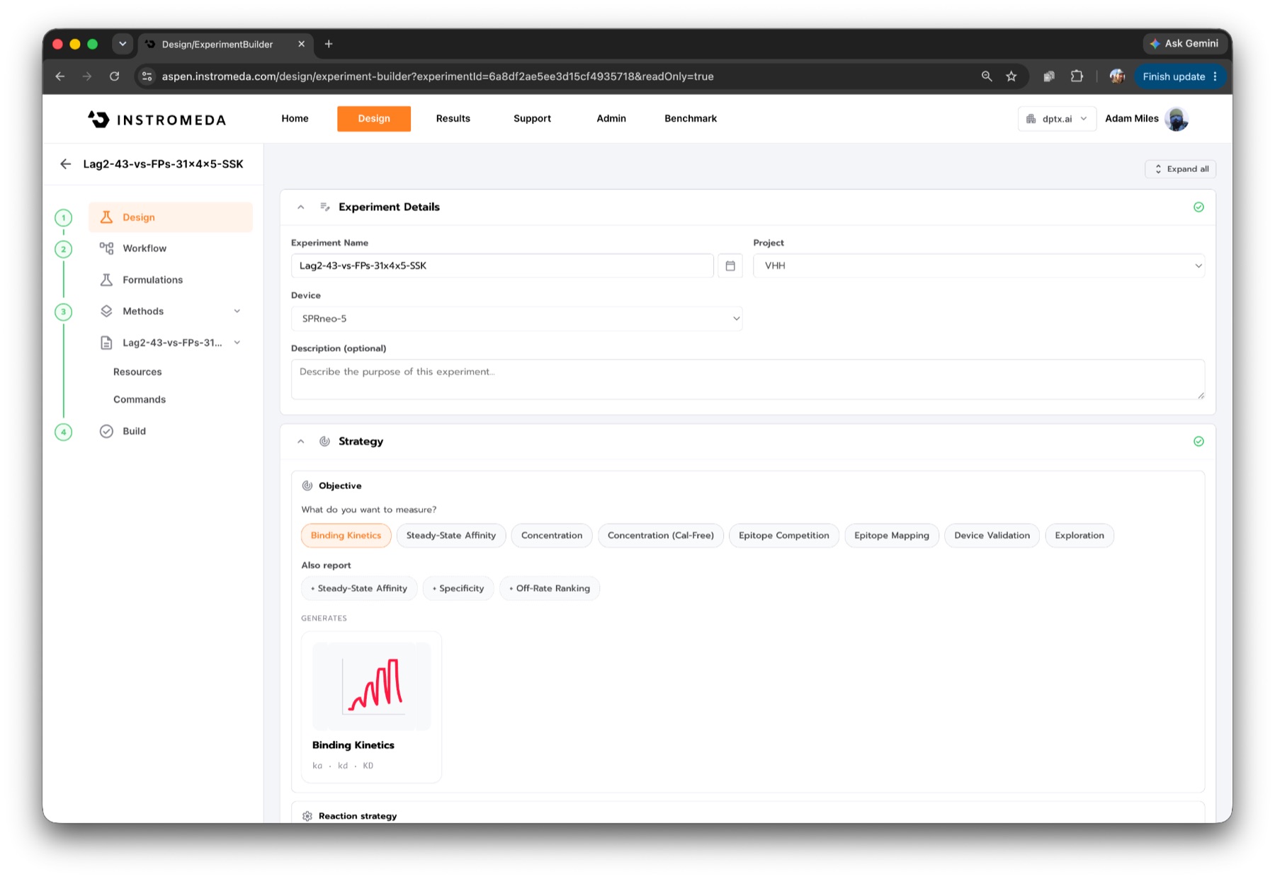
Design a single-cycle kinetics screen for 31 VHH-Fc constructs in mammalian
supernatant, captured on a Protein A/G chip (about 10 ug/mL each). Two of them
are negative controls: Fc only and an anti-HSA VHH-Fc. Analytes: sfGFP(DP0338),
eGFP(DP0339), ECFP(DP0340) and ECFP(DP0341), all about 31 kDa, each at 12.3 nM
to 1 uM in a 3-fold series (5 points). Device: SPRneo-5, 25 C.

Ligands (name, MW):
- Fc only (29.95 kDa) -- negative control
- aHSA-VHH-Fc (39.56 kDa) -- negative control
- LaG-2-3C-Fc (40.96 kDa)
- ... 28 more
From that one request the platform generated a three-activity method: a warmup to settle temperature and optics, surface conditioning chosen from the chip type (two pulses of glycine pH 1.5 on Protein A/G), and the capture-kinetics activity. In capture kinetics, each VHH-Fc is captured for 25 s, a buffer blank runs before each surface, all five concentrations of one target are injected in a single cycle (100 s association, 100 s gaps, 300 s final dissociation), and three short pulses of glycine pH 2.0 strip the surface. Evaluations were wired in automatically: baseline after warmup and conditioning, then capture and kinetics after the run.
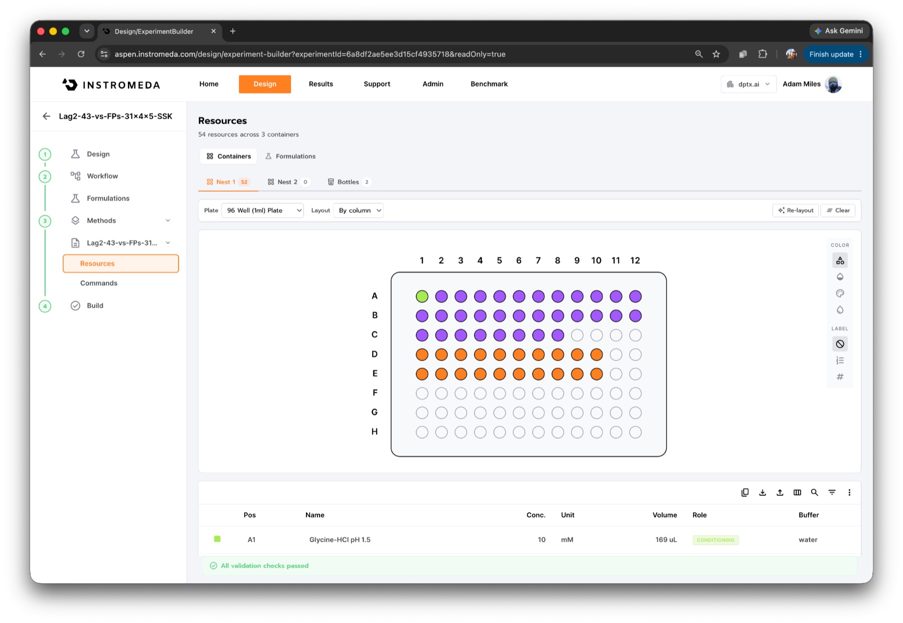
The plate the platform built for this screen held 54 resources across three containers, and every validation check passed before the run started.
The run
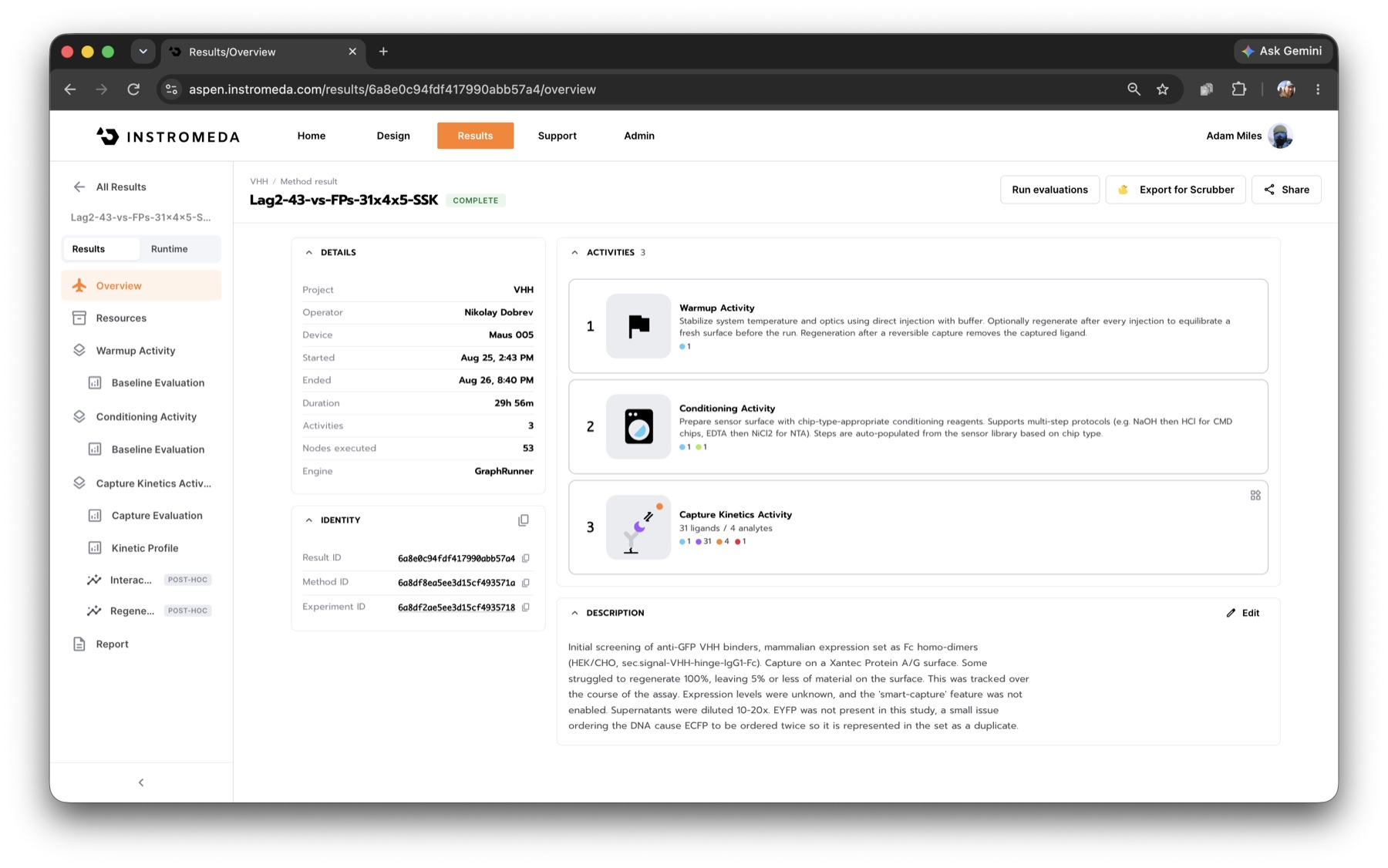
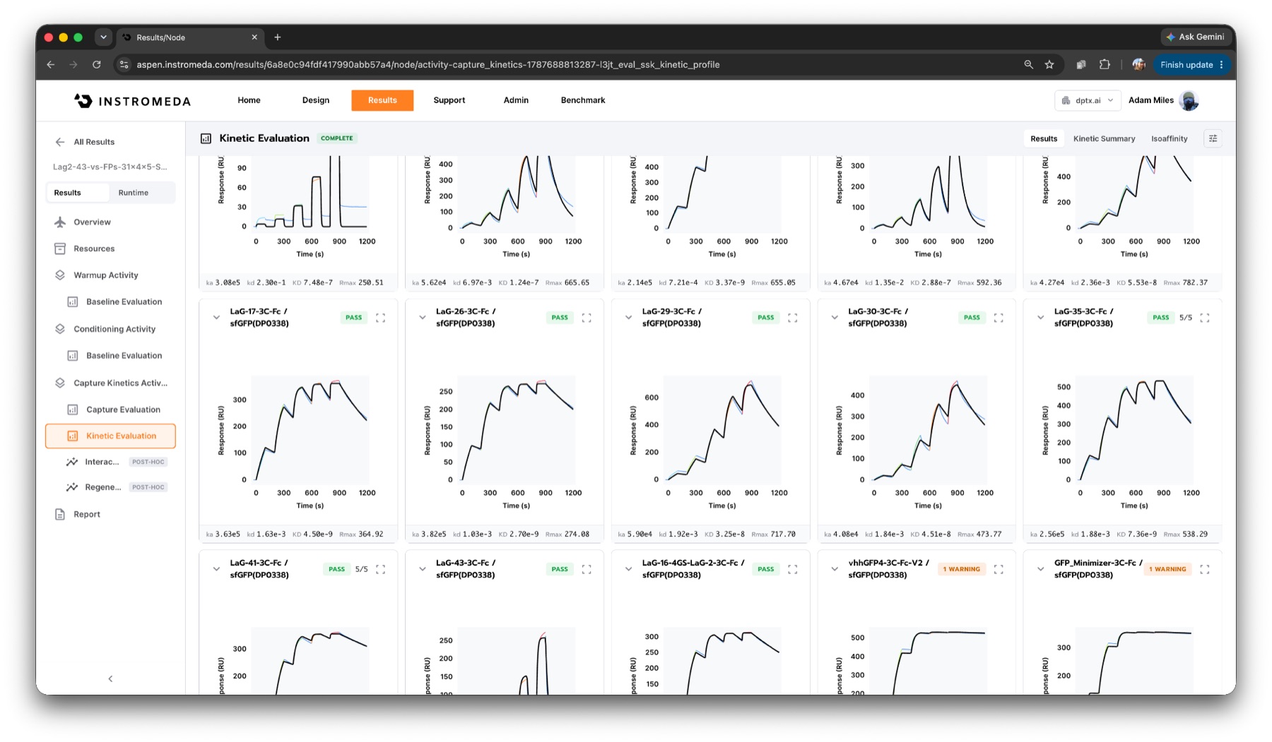
Nikolay started the run at DPtx on 25 August, and it finished 29 h 57 min later without anyone touching the instrument: about four interactions per hour. Each VHH-Fc was captured on a Protein A/G surface, and each target was titrated over it as single-cycle kinetics 11: five concentrations, 3-fold from 12.3 nM to 1 µM, with a 300 s final dissociation. Every channel was referenced against an uncaptured reference channel and a buffer cycle (double referencing 10).
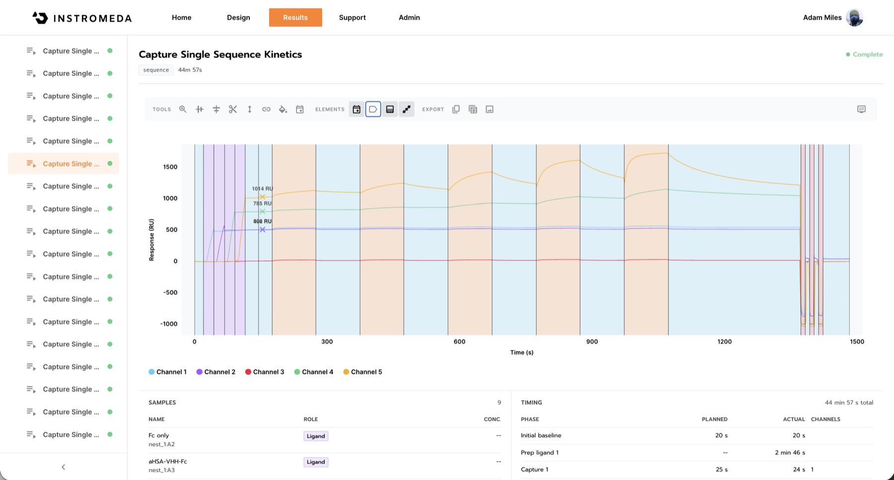
Each single-cycle sequence takes about 45 minutes: four ligands captured on four channels, five injections of one target over all of them, then regeneration. The raw view shows how differently the supernatants captured within one sequence, from about 500 to 1,014 RU.
Each interaction was fitted to a 1:1 model 8 and graded by a fixed set of checks: real signal, phase shape, fit quality, dose response, how well the parameters are determined, controls and residual trend. Each check's verdict is on record next to the number. The cards shown here come from a re-evaluation of the stored run with the current version of those checks.
The instrument analyzes each interaction as it completes. Fits and grades build up while the run is still going, so the science shows itself in real time, and the instrument, or an agent watching it, can respond to what it sees as the run unfolds.
Results
Run quality
The most useful internal check in this screen is ECFP, which was run as two independently prepared batches. Across the 23 ligands that gave a usable fit on both, the KDs agree to a median of 1.13x (worst 1.45x), with r² 0.997 over a range of about 2,700-fold. The off-rates agree even more closely, to a median of 1.02x. Capture was stable from cycle to cycle, at a median CV of 1.9%.
The off-rate being the most reproducible number is not an accident, and it comes up again below. Where an off-rate was too slow to measure within the 300 s dissociation, we report it as a limit (kd < 1.7 × 10⁻⁴ s-1) rather than a fitted value.
The interaction matrix
Of the 124 interactions, 98 produced a kinetic fit and 87 of those are usable (74 high confidence, 13 usable). Eleven fits were flagged not usable, 8 interactions showed only trace signal, and 18 were non-binders.
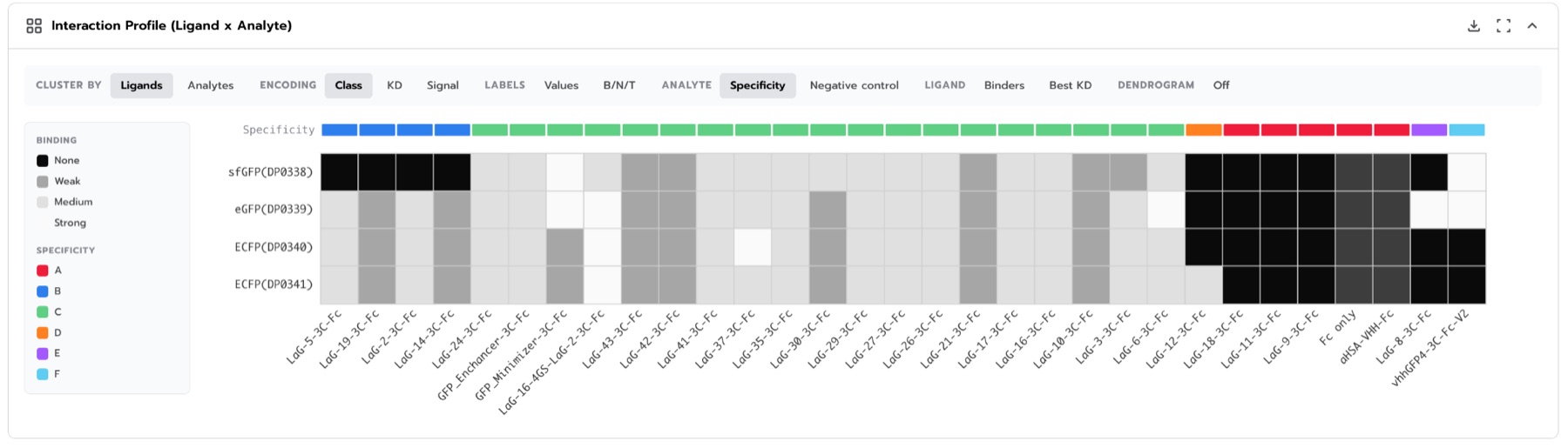
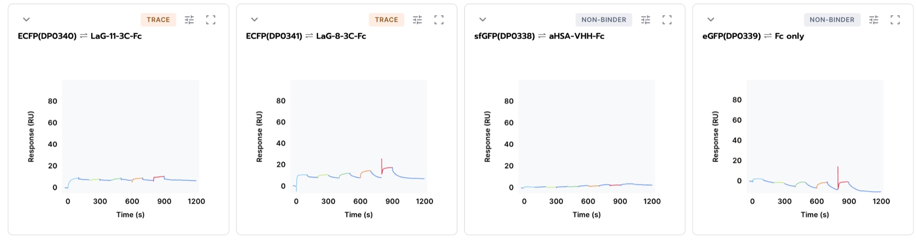
The anti-HSA control and LaG-18 were clean non-binders on all four targets. The Fc-only surface showed a trace signal on sfGFP, which the platform flagged as not a clean negative rather than passing it.
Weak binders get the same treatment. LaG-8 and LaG-11 were measured at around 20 µM in the original bead-binding assay 1. At our top concentration of 1 µM, a 20 µM binder occupies less than 5% of its sites, so a small, structured signal is what you should see, and the platform reports it as trace, with no KD, rather than forcing a fit onto it.
Specificity, and what the structures say about it
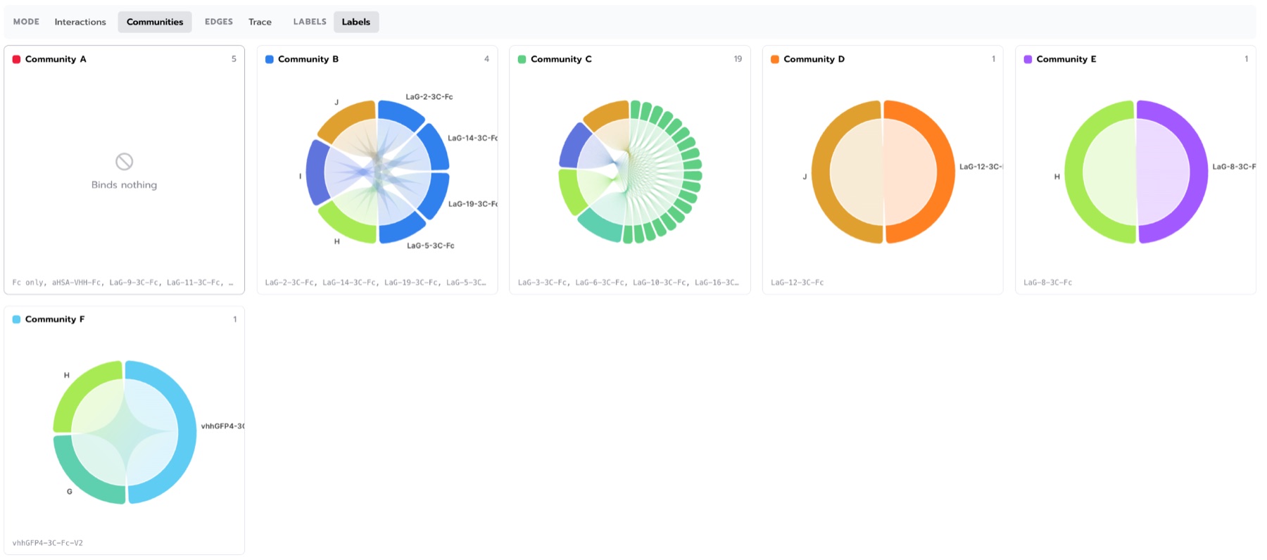
Clustering the ligands by their binding pattern across the four targets separates the panel by specificity. The clearest group is the clones that bind eGFP and both ECFPs but not sfGFP: LaG-2, LaG-24, LaG-27 and LaG-37. These communities are groups of shared specificity, not epitope groups: LaG-16 and LaG-30 share an epitope but differ 12-fold in affinity, for example.
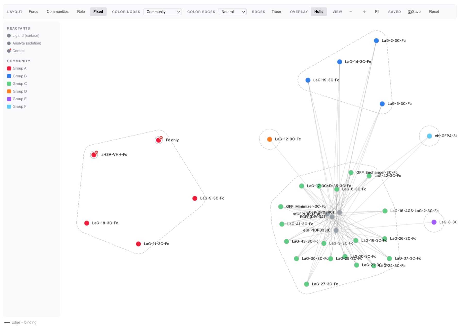
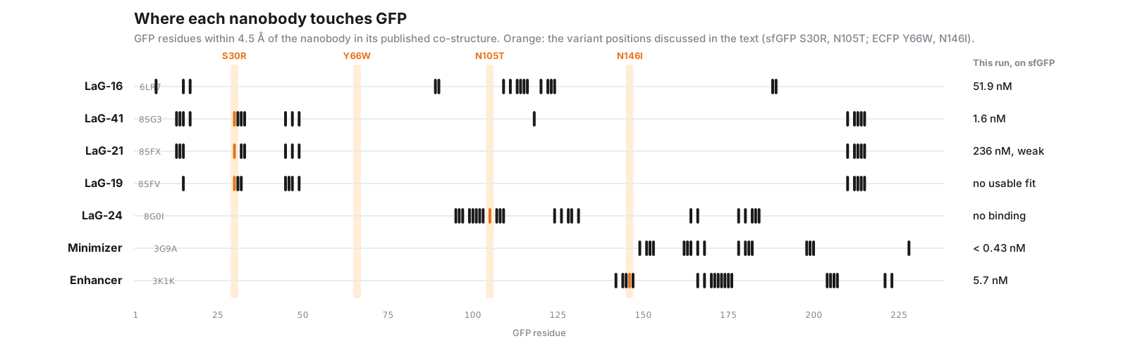
The original LaG study did not test sfGFP 1, so these dropouts are new. Several of them line up with the published co-structures 2 at the residue level. We recomputed the contacts from the deposited coordinates:
- LaG-24 contacts GFP Asn105 directly (4.4 Å, PDB 8G0I). sfGFP carries Thr at position 105. LaG-24 binds eGFP at 12.4 nM and both ECFPs, and does not bind sfGFP at all.
- LaG-19, LaG-21 and LaG-41 share one epitope (PDB 8SFV, 8SFX, 8SG3), and all three contact Ser30, another position sfGFP changes. That family is where sfGFP behavior splits: LaG-41 still binds sfGFP at 1.6 nM, LaG-21 only weakly (236 nM), and LaG-19 and LaG-42 give no usable fit on it.
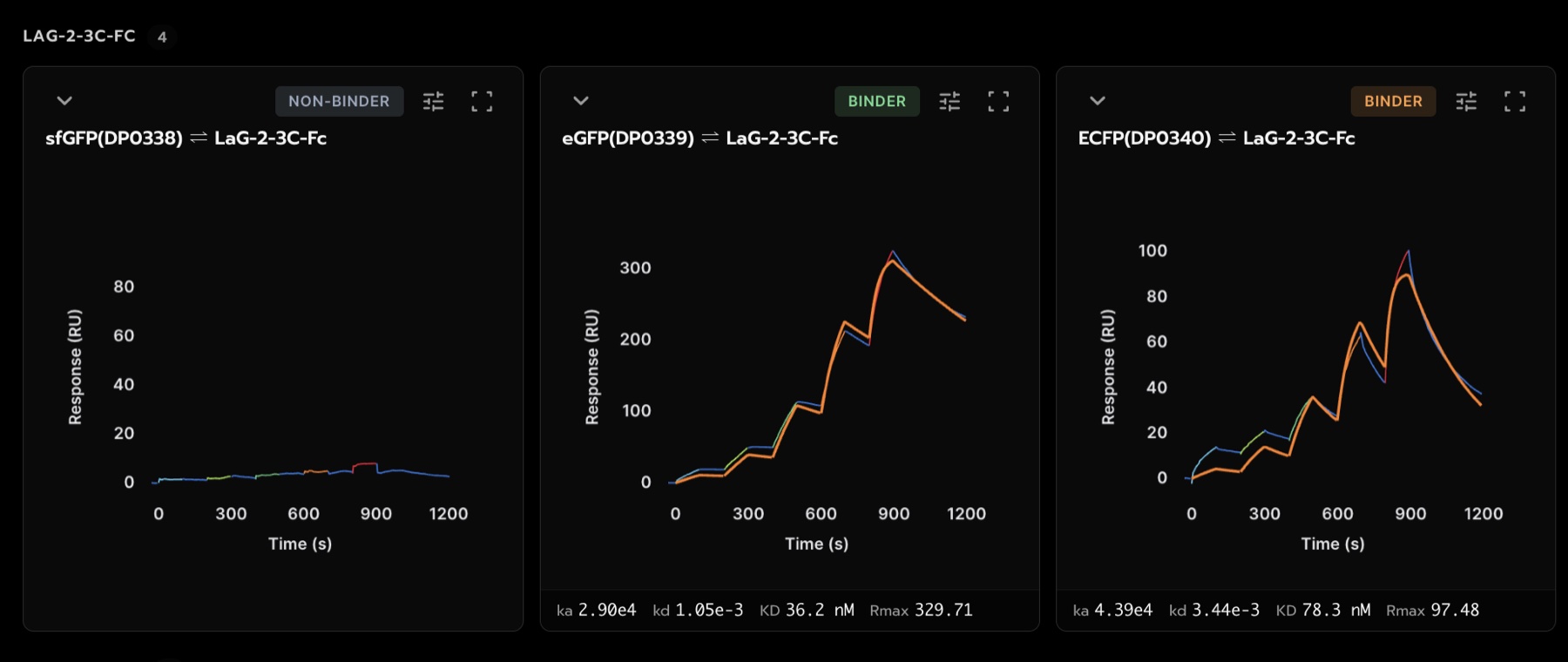
LaG-2 shows how much the variants can matter for a single clone. It does not bind sfGFP at all, binds eGFP cleanly at 36 nM, and binds ECFP at 78 nM but reaches only about a third of the eGFP signal (Rmax 97 RU against 330 RU). That drop is much larger than LaG-2's cycle-to-cycle capture variation, so on ECFP a smaller fraction of the surface is binding, not just binding more weakly.
A same-epitope affinity ladder
On eGFP the LaG-41 family gives a clean ladder at one epitope, all four fits high confidence: LaG-41 4.5 nM, LaG-21 197 nM, LaG-19 316 nM and LaG-42 788 nM, about 175-fold end to end. A series like this, with the epitope confirmed structurally, is useful for calibrating a scoring model. (These structures and mutants are now published 2, so this family is no longer held out from recent models.)
The Minimizer: tight on the GFPs, fast exchange on ECFP
The GFP Minimizer 4 binds sfGFP and eGFP with no measurable dissociation in 300 s (KD < 0.43 nM). On ECFP the same molecule turns into a fast-on, fast-off binder with an apparent KD near 700 nM, more than a thousand-fold weaker. Nearly all of that difference is in the off-rate: at least 760-fold, and the true value is larger because the GFP side is below the measurable floor.
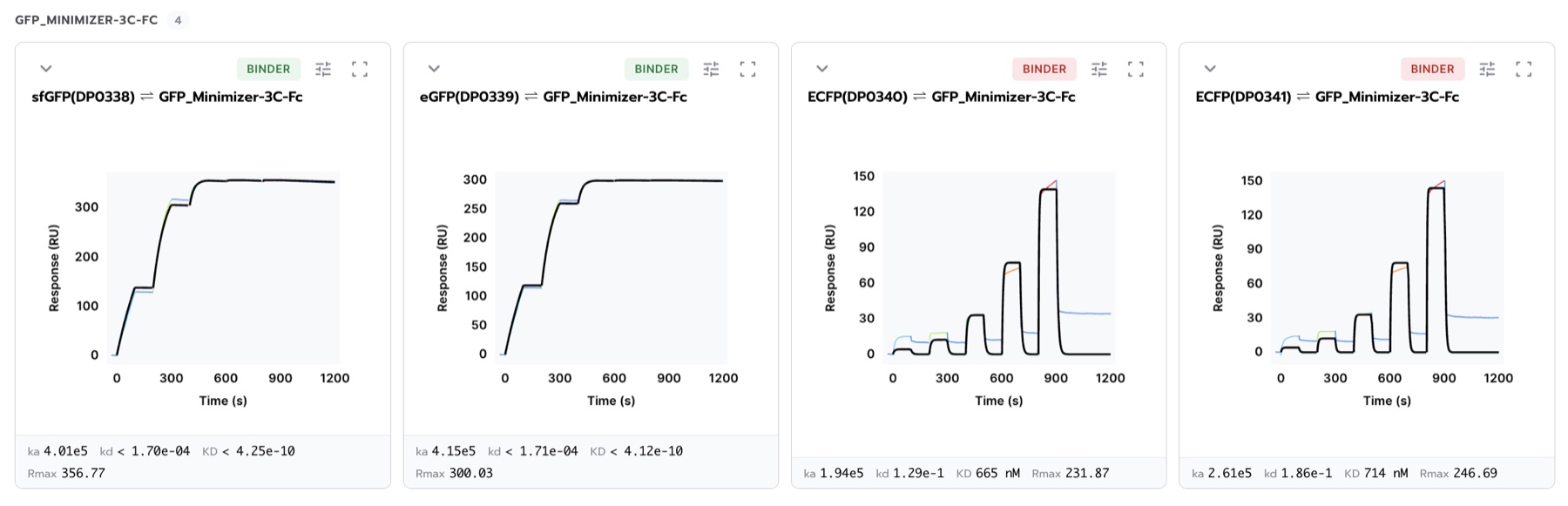
The only positions where ECFP differs from both GFPs are the chromophore (Y66W) and one surface position (N146I). In the Minimizer co-structure (PDB 3G9A) the nanobody sits about 10 Å from the chromophore and contacts neither residue, so this looks like an indirect, conformational effect, consistent with what Kirchhofer and colleagues described for the Minimizer 4. The ECFP fits are flagged as multiphasic, so treat the 700 nM as approximate. A steady-state fit would suit this shape of data better.
Selected kinetics
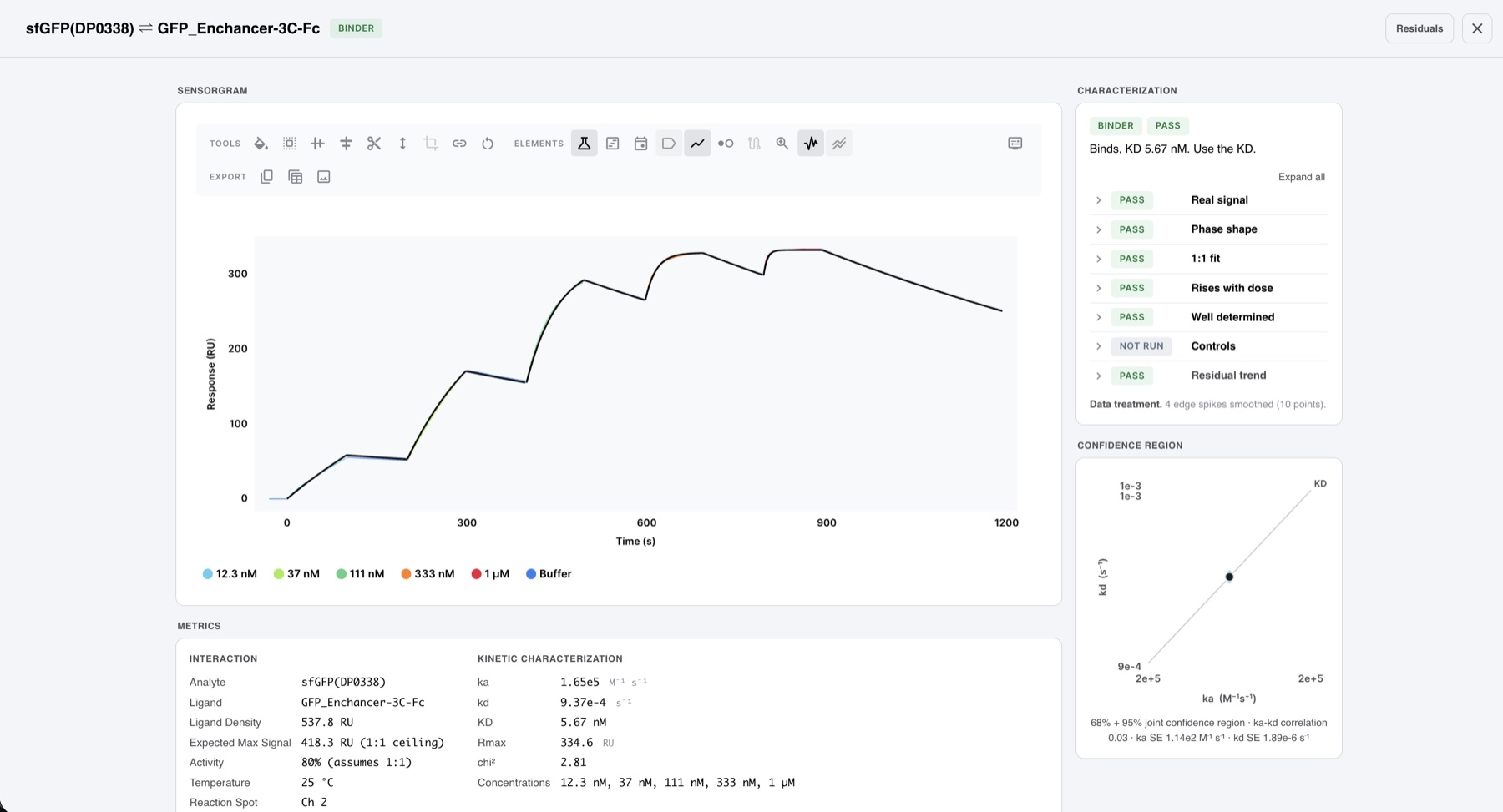
The GFP Enhancer on sfGFP is one of the cleanest interactions in the panel: KD 5.67 nM, 80% activity, and every check that applies passing.
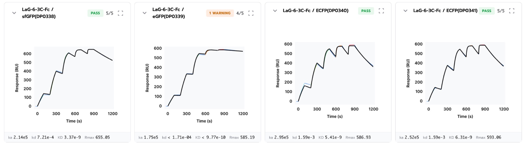
LaG-6 binds sfGFP at 3.3 nM, and the two ECFP batches give 5.2 and 6.2 nM.
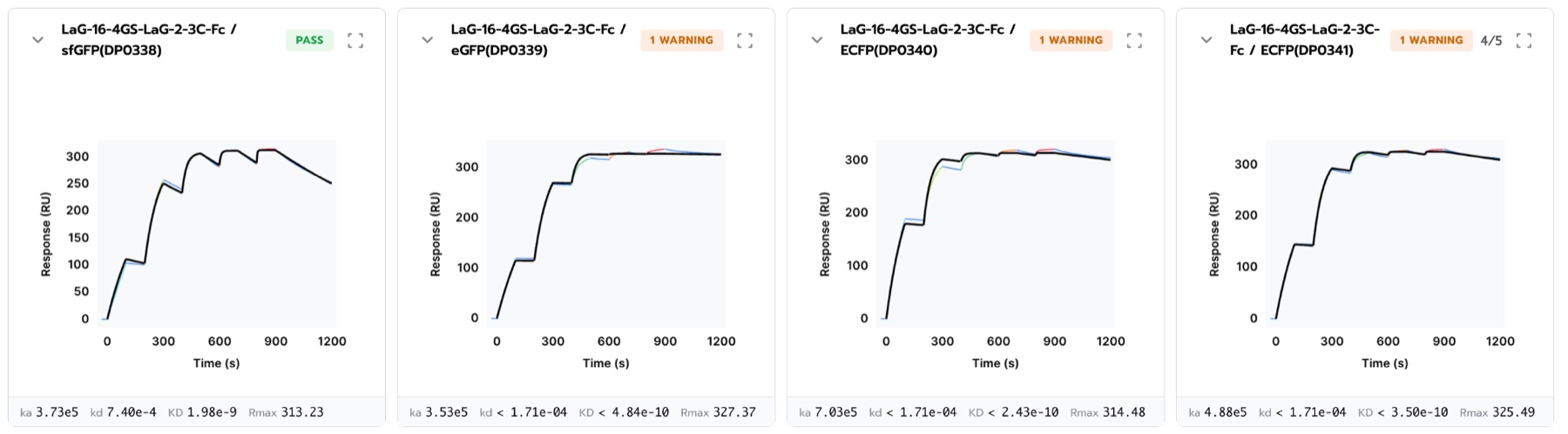
The LaG-16-LaG-2 tandem binds sfGFP at 1.96 nM, 26-fold tighter than LaG-16 alone (51.9 nM). On the other three targets its off-rate is below the measurable floor.
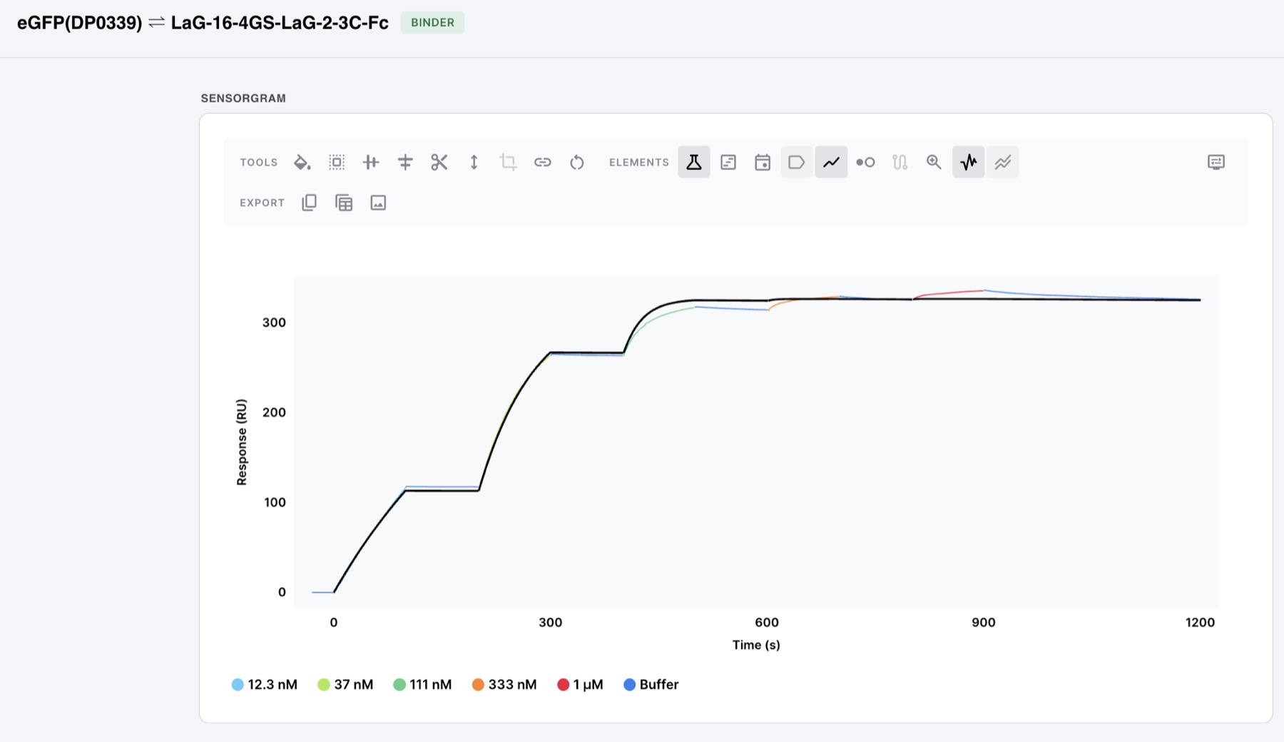
The tandem's two halves explain its two behaviors. LaG-2 on its own does not bind sfGFP, so on sfGFP the tandem behaves essentially as LaG-16 and fits a clean 1:1 model. On eGFP both halves bind (LaG-2 alone at 36 nM), and the curve shows what two linked binding sites look like: fast saturation and no measurable dissociation, which a 1:1 model cannot fully describe at the higher concentrations. That the tandem still gains 26-fold on sfGFP suggests LaG-2 keeps a contact too weak to see on its own, which the linked format turns into avidity. That last point is our interpretation, not a measurement. The signal here peaks around 330 RU: fine for SPR, though below 200 RU would be better for kinetics.
Comparison with published affinities
Our format is the reverse of the original study's. Fridy and colleagues amine-coupled GFP to the chip and flowed the nanobody 1. We captured the VHH-Fc by its Fc and flowed untagged GFP. Our orientation keeps the target free in solution, so random amine coupling cannot block lysine-containing epitopes (the LaG-41 family's epitope includes two lysines). But our capture densities were uncontrolled, and high density slows the apparent on-rate through mass transport 9. Neither format is ground truth, so the fair comparison is the off-rate.
| Clone | Published KD (nM) 1 | This run, eGFP (nM) | Ratio |
|---|---|---|---|
| LaG-37 | 24 | 25.3 | 1.1x |
| LaG-42 | 600 | 788 | 1.3x |
| LaG-10 | 97 | 145 | 1.5x |
| LaG-3 | 25 | 58.9 | 2.4x |
| LaG-29 | 110 | 60.0 | 0.55x |
| LaG-41 | 0.9 | 4.5 | 5.0x |
| LaG-16 | 0.7 | 42.8 | 61x |
| LaG-30 | 0.5 | 511 | ~1,000x |
Most clones agree within about 2.5-fold, despite the different orientation and instrument. A few do not. LaG-16 had the highest capture level in the run, 1,582 RU, which is exactly where we would expect mass transport to compress the on-rate. LaG-30 is the one we cannot yet explain. Our own data on it is self-consistent: on eGFP and both ECFP preparations it is a fast-on, fast-off binder (356 and 347 nM on the two ECFP batches, 511 nM on eGFP), and the shape of the dose response gives the same answer without any kinetic fit. A 0.5 nM binder would already be about 96% saturated at our lowest concentration (12.3 nM), so all five steps would reach nearly the same height; ours roughly double between 333 nM and 1 µM, as a binder near 500 nM should. On sfGFP the same clone binds ten-fold tighter (43 nM). We are checking our LaG-30 construct against the published sequence. On the off-rate, our LaG-41 (1.34 × 10⁻³ s-1) is within 1.4-fold of the Rout lab's value for a LaG-21 variant they describe as on par with LaG-41 2, while the on-rates differ about ten-fold. Off-rates transfer between labs; on-rates are much more sensitive to format.
This run also gives the first SPR values for LaG-19 and LaG-35, which were previously measured only by bead-binding assay 1.
Notes on the data
This was a first screen, set up quickly to get the panel started. SPR specialists will likely spot the following.
- Surface density was not controlled. Supernatant capture gave a 57-fold spread in capture level, some surfaces sit at high Rmax, and on-rates fall with density. Treat these KDs as apparent, and rank on the off-rate.
- This is one format of several. The Fc fusions on Protein A/G are the mammalian arm of the expression comparison, used here to check the reagents. Bivalent ligand with a monovalent analyte behaves as 1:1, but the affinities we would stand behind come from the Twin-Strep formats on StrepTactin XT with controlled capture.
- Ligand preparation matters more than the instrument. vhhGFP4 and the GFP Enhancer are the same nanobody 4, 5, here from two preparations, and they differ more than 10-fold on sfGFP. That is the largest source of error in this screen, and it is on the reagent side.
- Protein A/G was not our preferred capture surface. It carried some non-specific background that did not fully regenerate. Our standard for Fc fusions is an anti-human Fc capture antibody (Jackson ImmunoResearch), the surface most published Fc-capture work uses, and it regenerates more cleanly. The follow-up on this set will use it.
- Smart capture came later. Capture-to-target was not ready for this run.
In short: the data is good and usable, and 87 of 124 interactions gave a usable fit. The next improvements are an anti-human Fc capture surface and a lower, controlled surface density, which is exactly what smart capture does.
Next: capture to target
Smart capture loads the surface in steps toward the density the assay calls for. In a follow-up run at DPtx, a Twin-Strep-tagged HSA was loaded at four concentrations spanning 10-fold (10 to 100 µg/mL) against a 500 RU target. All four surfaces landed between 422 and 445 RU. An anti-HSA VHH titrated over each gave KD 4.3 to 6.4 nM, a confirmed 1:1 fit on every surface, Rmax 61 to 75 RU, and 100% regeneration recovery. The whole run took 2 h 10 min.
Capture time is not fixed. The instrument watches each channel and stops loading when it reaches the target: the first capture here was planned for 2 minutes and stopped at 63 s, and the dashed lines mark the 500 RU target on every channel.
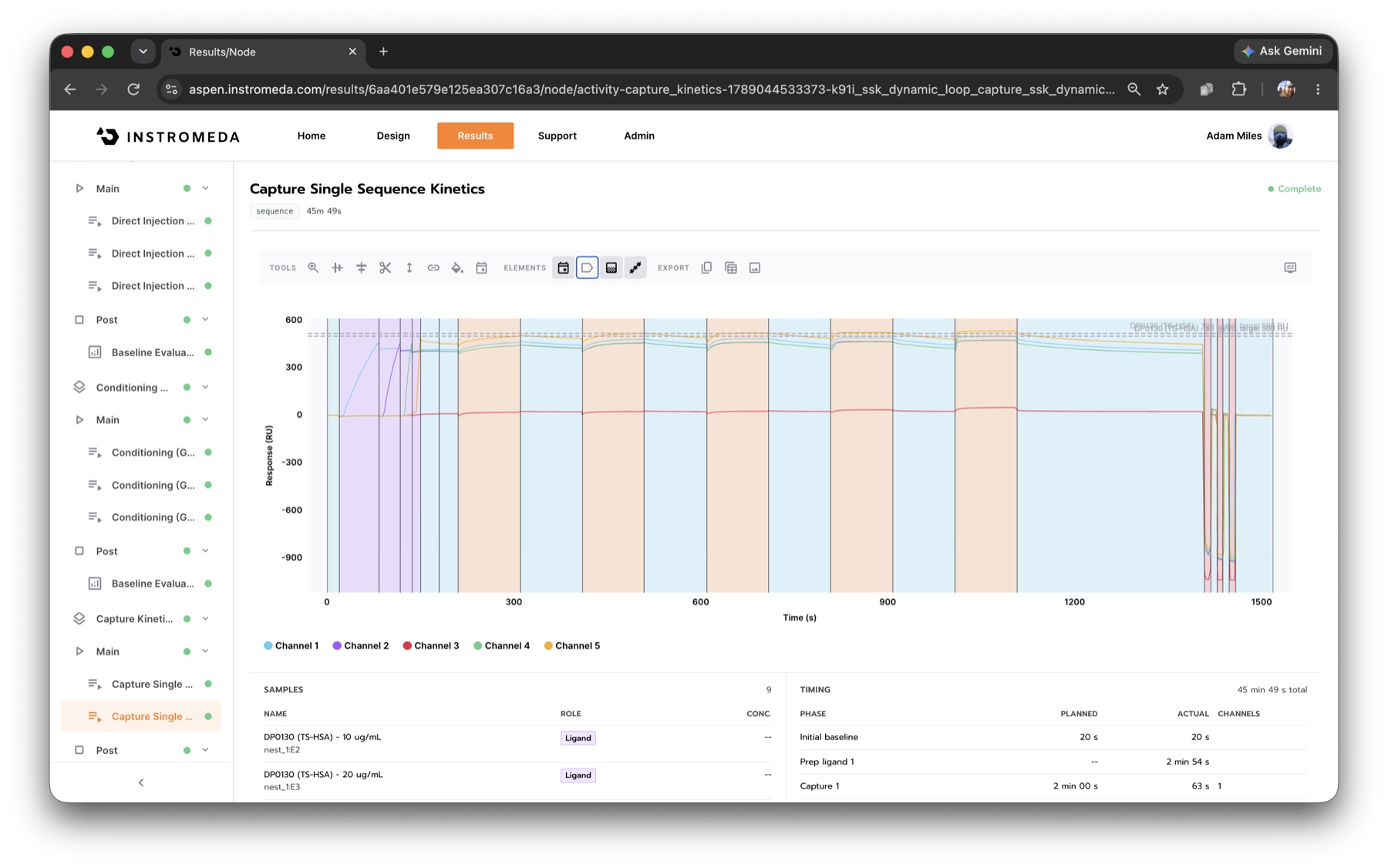
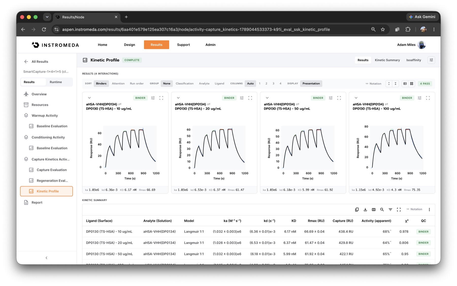
The next round of the panel will use this format, followed by designed binders against the same targets.
Agents: a tool-shaped instrument
Agents that design and run experiments are arriving quickly, and the hard part is grounding them in the physical lab. Google Research recently described what that took on general-purpose lab robots: a "semantic digital twin" that tracks the live physical state of the workcell, because current models "still do not reason reliably about 3-dimensional geometry and physical state", and a virtual dry run of every protocol before it touches reagents 12. With that in place, their agents closed the design-test loop on DNA aptamers and de novo protein binders.
We approach the same problem from the instrument side. SPRneo owns the physical layer outright: fluidics, scheduling, capture, regeneration and data quality. An agent never has to reason about a flow path or a pipette. It works at the level of the science: what to measure, which reagents, what came back and what to do next. The instrument's preview run checks a design before anything is run, and every result comes back graded, with the rule behind each verdict. We think of this as an instrument that is tool-shaped: its operations are ones an agent can understand and call directly.
Most current models already know a good deal of SPR science: binding models, mass transport, regeneration, how to read a sensorgram. What they lack is a way to act on that knowledge. What they need is an instrument that gives them a framework: explicit operations for design, execution and analysis, results they can trust and read back, and a clear contract at each step. The same experiment the web builder produced here can be requested by an agent over MCP, by a lab system over SiLA 2, or by a script over REST, as in the Methods.
Two approaches are common today. One is to build a software layer around an instrument after the fact. The other is to expose an API and leave the rest to whoever calls it. Agents are good at reading a codebase and can often make that work, but it is never as efficient for them as an instrument designed with them in mind. We think it is the instrument maker's job to treat agents as first-class users and design for them as carefully as for people. Code is close to being the common language of automated biophysics, but it should not have to be. With an instrument built this way, you put it on the bench and it works with your people, your informatics and your agents from day one.
We have had agents run SPR on SPRneo end to end: design the experiment, start it, watch it run, and report the results, with the instrument helping as much as needed while the agent does the work and steers. We will publish those end-to-end runs soon.
Twelve models, one experiment
We gave twelve current language models from seven developers, from frontier models to small open-weight ones, the request a scientist would type for this experiment: a single-cycle kinetics screen for 31 VHH-Fc constructs captured on Protein A/G, with two negative controls and four fluorescent-protein analytes. Each model worked only through the SPRneo MCP server, and the platform checked every design in a preview run that saves nothing. 10 of the 12 models produced a correct design in all three of their tries, and 30 of 38 runs passed every check. A passing design took a median of 2 tool calls, about 44,000 tokens and 40 seconds, and cost about 5 US cents.
| Model | Correct designs | Tool calls | Tokens (median) | Cost per design |
|---|---|---|---|---|
| Claude Opus 5.5 | 3 of 3 | 2 | 44k | $0.25 |
| Claude Sonnet 5.5 | 3 of 3 | 2 | 44k | $0.12 |
| Claude Haiku 5.5 | 3 of 3 | 2 | 47k | $0.007 |
| GPT-6.1 | 3 of 3 | 3 | 39k | $0.03 |
| GPT-6 luna | 3 of 3 | 2 | 34k | $0.004 |
| Gemini 4 Argon | 3 of 3 | 2 | 28k | $0.06 |
| Gemini 3.8 Flash | 3 of 3 | 3 | 39k | $0.03 |
| DeepSeek v4.1 Flash | 3 of 3 | 3 | 34k | $0.003 |
| Mistral Large 4 | 3 of 3 | 3 | 56k | $0.05 |
| Qwen 3.8 Max | 3 of 3 | 5 | 83k | $0.31 |
| Gemma 4 31B | 0 of 3 | 1 | 14k | |
| Llama 4 Maverick | 0 of 5 | 0 to 1 |
The usual path is short: read the allowed values, then send one request with all 35 reactants. The platform chooses the activities, the schedule and the regeneration. About 90% of the tokens are the framework the platform provides (tool descriptions, domain knowledge and its replies); the model's own output, the request itself, is a few thousand. The validation errors do real work: one model sent malformed arguments in every run, read the platform's error, and corrected itself each time. The two models that failed ignored the chip named in the request, and one could not issue tool calls reliably.
A design passes when it has the right strategy, chip, ligands, controls, and four distinct analytes with the right concentration series. Analyte names may repeat (two batches both called ECFP), because the platform identifies samples by id; scored on exact names instead, 19 of 38 runs pass, and nothing else changes. Three tries per model is a small sample, and the request names the chip and lists every reagent, so this tests turning a request into a correct, executable design rather than choosing the strategy. Run on 19 October 2026 through OpenRouter, which is also where the costs come from.
A first look at the alternative
In a small pilot, we gave five of the same models only the raw REST API and its specification instead of the MCP server. Three did as well as before; two did worse, and 11 of 15 runs passed, against 15 of 15 through MCP. Passing runs cost about the same. The failures are the instructive part. One model left out the strategy, and the API, which fills in defaults, returned a successful design for the wrong chemistry. An interface for agents should refuse what it cannot do correctly and say why, rather than guess. We are fixing that, and the full benchmark will include this comparison. This is a pilot: one task, three runs per model.
This is a teaser for a benchmark we run regularly. Our goal is to lower the floor: make the instrument usable by as many agents as possible, not only the largest models. Each round tells us where agents stumble, and we change the platform rather than the prompt. The two open-weight models that failed here are the next target. We have been building SPRneo for agents for the past year, and a full benchmark of agents designing, running and analyzing SPR experiments, and of what it takes to build instruments for them, will follow.
Where people fit
Customers often tell us what they think experts will make of an instrument like this. Our honest view is that it replaces the busy work, not the scientist: watching a run by hand, the missed lunch spent getting an assay to work, staying late to start one more overnight run because one last condition needs optimizing. No more late nights at the lab, at least not because of SPR. Let the instrument do what machines are good at, and let agents do what they are good at. In this screen no one needed SPR expertise to design the assay, run it for 30 hours or grade 124 interactions. The interesting parts of this note are where people did engage: recognizing that the tandem binds in two linked steps, deciding whether LaG-30's 500 nM is real, connecting the Minimizer's off-rate to a structure 10 Å away. This is also what opens SPR to generalist scientists. A biologist who is not an SPR specialist should be able to say what they want to know about a set of interactions and let their agent do the rest. Agents already know enough of the science; what decides whether it works is the instrument. When the instrument is legible, even small, inexpensive models design the experiment correctly, and the results come back graded, with the reason for each verdict, so the scientist can trust them without reading sensorgrams the way a specialist would. We think we are entering the age of the generalist, and that is the real promise of agents: more people succeeding with data like this, not just agents.
We are building toward agentic scientists: agents that take a question, design the experiment, run it on an instrument like this one, read the results and decide what to do next, with people setting direction and judging what matters. In our workshop we regularly watch agents design and run experiments on SPRneo. This note lays out the pieces, and we will follow it with the full workflow and its demonstration over the course of this project, and many more to come. That frees scientists for the bigger questions, and it produces more high-quality data, at a scale no one could run by hand.
Acknowledgements
Thank you to Dr. Nikolay Dobrev and the DPtx team for producing the reagents, running the instrument and for the collaboration.
Contact
DPtx (Data-Powered Therapeutics): Dr. Nikolay Dobrev, CEO, nikolay@dptx.ai · partnerships info@dptx.ai · dptx.ai
Instromeda: contact us · SPRneo
References
- Fridy PC, Li Y, Keegan S, et al. A robust pipeline for rapid production of versatile nanobody repertoires. Nat Methods. 2014;11(12):1253-1260. doi:10.1038/nmeth.3170
- Ketaren NE, Fridy PC, Malashkevich V, et al. Unique mechanisms to increase structural stability and enhance antigen binding in nanobodies. Structure. 2025;33(4):677-690.e5. doi:10.1016/j.str.2025.01.019
- Rothbauer U, Zolghadr K, Tillib S, et al. Targeting and tracing antigens in live cells with fluorescent nanobodies. Nat Methods. 2006;3(11):887-889. doi:10.1038/nmeth953
- Kirchhofer A, Helma J, Schmidthals K, et al. Modulation of protein properties in living cells using nanobodies. Nat Struct Mol Biol. 2010;17(1):133-138. doi:10.1038/nsmb.1727
- Kubala MH, Kovtun O, Alexandrov K, Collins BM. Structural and thermodynamic analysis of the GFP:GFP-nanobody complex. Protein Sci. 2010;19(12):2389-2401. doi:10.1002/pro.519
- Pédelacq JD, Cabantous S, Tran T, Terwilliger TC, Waldo GS. Engineering and characterization of a superfolder green fluorescent protein. Nat Biotechnol. 2006;24(1):79-88. doi:10.1038/nbt1172
- Heim R, Tsien RY. Engineering green fluorescent protein for improved brightness, longer wavelengths and fluorescence resonance energy transfer. Curr Biol. 1996;6(2):178-182. doi:10.1016/S0960-9822(02)00450-5
- Myszka DG. Kinetic analysis of macromolecular interactions using surface plasmon resonance biosensors. Curr Opin Biotechnol. 1997;8(1):50-57. doi:10.1016/S0958-1669(97)80157-7
- Myszka DG, He X, Dembo M, Morton TA, Goldstein B. Extending the range of rate constants available from BIACORE: interpreting mass transport-influenced binding data. Biophys J. 1998;75(2):583-594. doi:10.1016/S0006-3495(98)77549-6
- Myszka DG. Improving biosensor analysis. J Mol Recognit. 1999;12(5):279-284. doi:10.1002/(SICI)1099-1352(199909/10)12:5<279::AID-JMR473>3.0.CO;2-3
- Karlsson R, Katsamba PS, Nordin H, Pol E, Myszka DG. Analyzing a kinetic titration series using affinity biosensors. Anal Biochem. 2006;349(1):136-147. doi:10.1016/j.ab.2005.09.034
- Rao P, Sirkovic P, Pawlosky A. Grounding AI agents in biological reality: building blocks for autonomous wet labs. Google Research blog, 16 October 2026. research.google/blog
- Law D, Kamichetty H. Progressable binders: the binders that matter. Xaira Therapeutics, 29 June 2026. xaira.com
- Boltz Team. A note on de novo binder design model evaluation. Boltz, 16 June 2026. boltz.com
- Anthropic. Claude protein binder design dataset: wet-lab notes (WETLAB.md). Hugging Face. huggingface.co
- OpenBind. Affinity and kinetics data in the EV-A71 2A OpenBind release. 5 May 2026. openbind.uk